- Innovations
- Articles on application of PCI
- Portfolio Trading
Portfolio Optimization through PQM Method (Part 1)
Searching for an optimal structure of assets in a portfolio is, by all means, not a simple issue. On the one hand, much depends on the parameters of the assets, included in the portfolio and on the other hand, on investor’s individual preferences and restrictions. However, modern financial theory and new analysis and trading methods considerably simplify that process.
Portfolio Quoting method can serve as an example of modern portfolio theory implementation, which allows constructing and analyzing numerous variations of portfolios, created from a wide range of assets. And the value of analysis capabilities lies in not only following the changes in the absolute price of the portfolio but also in studying the behavior of the portfolio in relation to the whole market or, for example, to an alternative portfolio, which allows making investment decisions in a timely manner. The result of the method appliance comes to be the creation of a new financial unit – synthetic instrument (with the technical name PCI – personal composite instrument).
In this article we will focus on a set of 6 US stocks, which at first sight have shown relatively good results in recent years. Through GeWorko method we have built a portfolio, showing considerable growth in the post - crisis period. Our selection (with corresponding random weights) consists of:
- Walt Disney Company (DIS – 20%)
- Home Depot Inc. (HD – 20%)
- Honeywell International Inc. (HON – 15%)
- International Business Machines Corporation (IBM – 15%)
- Coca-Cola Company (KO – 10%)
- McDonald’s Corporation (MCD – 20%)
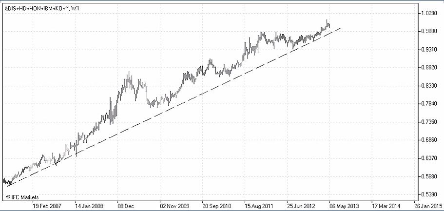
While comparing the portfolio dynamics with the market (Dow Jones Industrial Average index conditionally stands for the market and includes all the listed stocks) it turned out that the portfolio has been systematically outperforming the index before the crisis, during the crisis and in the period of its recovery. The PCI chart, formed within seconds, successfully illustrates the behavior of the portfolio in relation to the index:

In spite of quite successful random selection of weights in the portfolio, we do not yet know if it is optimal, i.e. if other weight coefficients exist there, providing lower risk at the same level of return, or higher return at the same risk level. If we manage to find such a portfolio it would certainly be more preferable for a rational investor than the portfolio with random weight coefficients. However, determining the portfolio optimality for an investor, as has already been mentioned above, will depend on individual preferences and restrictions. Without concrete requirements for the portfolio risk-return profile we cannot know if, for example, a portfolio with a higher return but also with a higher risk level is more preferable for the investor than the primary one. In this regard, for analytical purposes, an optimal portfolio will be considered the one that has the maximum return per unit of risk. That index is known as the Sharpe ratio.
In contrast to its traditional version, which shows the relation of risk premium above risk-free rate to standard deviation, we will maximize the relation of portfolio return to portfolio standard deviation, without adjusting for risk-free rate. That simplification will in no way influence the conclusions, which will allow comparing the effectiveness of alternative investment portfolios.
At first, let us return to the primary portfolio with randomly given weights and determine its parameters of risk and return. Portfolio analysis will be based on monthly data of closing prices of six stocks on the sample of January 2005 – April 2013. Since the initial aim was to compare the dynamics of the portfolio with the index (the market), we have decided to apply a slightly nonstandard approach and to adjust monthly closing prices of stocks, dividing them by corresponding index values. On the basis of logarithmic returns we have calculated mean returns and standard deviations of returns for six rows of data. The calculation results are presented in the table below:
Table 1: Mean returns, standard deviations and Sharpe rations for six rows of data
| DIS | HD | HON | IBM | KO | MCD | |
| Mean Return | 0.49% | 0.24% | 0.40% | 0.42% | 0.35% | 0.77% |
| StDev | 4.25% | 5.73% | 4.51% | 4.53% | 3.95% | 4.09% |
| Sharpe Ratio | 0.11 | 0.04 | 0.09 | 0.09 | 0.09 | 0.19 |
It turned out that the greatest (0.77%) monthly mean return (in comparison with the index) has been shown by MCD stocks, the smallest - by HD stocks (0.24%). The smallest standard deviation has been shown by KO stocks (3.95%), the greatest – by HD stocks (5.73%). Besides, we have calculated the simplified version of the Sharpe ratio, showing the relation of asset return to risk. MCD stocks have the highest coefficient (0.19), showing the best ratio of return per unit of risk. This fact allows us to assume that it is MCD stocks that will show the highest weight coefficient in an “optimal” portfolio. To continue the analysis, we will also need to know how the assets are interrelated – covariance coefficients will be used. The covariance matrix is calculated on the same sample of monthly data.
Having all the necessary input parameters and supposing that the obtained values of return and standard deviation for six stocks come to be the best estimations of expected returns and risks, we can start forming portfolios. Recall that input data have already been adjusted for the index value. That is why the portfolios that we should obtain will already reflect the behavior in relation to the market.
The first portfolio (P1) will become the starting point for searching for more successful combinations of assets. It is the portfolio with random weight coefficients; its price chart has been presented in the very beginning. Knowing the risk and return parameters of six stocks, included in the portfolio, their weights and the covariance matrix, we can calculate the monthly mean return of the portfolio and its standard deviation. It is easy to notice that by means of combining assets we have achieved a significant reduction of risk. The standard deviation of portfolio P1 is only 1.74% and the return is – 0.46%:
Table 2: Realized returns, standard deviations and Sharpe ratios in relation to portfolio P1
| DIS | HD | HON | IBM | KO | MCD | P1 | |
| Mean Return | 0.49% | 0.24% | 0.40% | 0.42% | 0.35% | 0.77% | 0.46% |
| StDev | 4.25% | 5.73% | 4.51% | 4.53% | 3.95% | 4.09% | 1.74% |
| Sharpe Ratio | 0.11 | 0.04 | 0.09 | 0.09 | 0.09 | 0.19 | 0.26 |
Additionally, in comparison with any of the six stocks, the portfolio has higher return per unit of risk, the evidence of which is the Sharpe ratio (0.26), which will ultimately determine the effectiveness of the portfolio.
Now, knowing the random portfolio features, we can start searching for such a combination of assets, that will best correspond to our preferences and restrictions. As has already been mentioned, we have chosen the Sharpe ratio as the basic criterion of optimality. Changing the weights of the six stocks that form the portfolio, we should find such a combination, which will correspond to the highest possible ratio of return to risk. The only optimization conditions we set is that weight coefficients should be not less than zero, and their sum should be equal to 100%, so as to keep the opportunity of comparing portfolios.
The solution leads us to the following composition of the portfolio: as we have expected, MCD stocks have got the greatest weight (32.67%), since they had the highest Sharpe ratio. Then come the following stocks in weight descending order: DIS (19.33%), HON (19.04%), HD (10.96%), KO (10.28%) and IBM (7.71%):
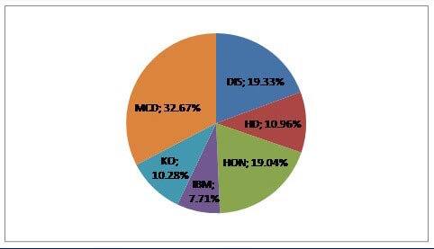
As a result, the portfolio (P2), obtained by changing the weights to maximize the Sharpe ratio, showed clearly better performance than the portfolio with random weight coefficients (P1):
Table 3: Realized returns, standard deviations and Sharpe ratios in relation to portfolios P1 and P2
| DIS | HD | HON | IBM | KO | MCD | P1 | P2 | |
| Mean Return | 0.49% | 0.24% | 0.40% | 0.42% | 0.35% | 0.77% | 0.46% | 0.52% |
| StDev | 4.25% | 5.73% | 4.51% | 4.53% | 3.95% | 4.09% | 1.74% | 1.72% |
| Sharpe Ratio | 0.11 | 0.04 | 0.09 | 0.09 | 0.09 | 0.19 | 0.26 | 0.30 |
The maximized Sharpe ratio was 0.3 for P2. This value is higher than the ratio for P1 (0.26)and for individual stocks. Moreover, both return (0.52%) and standard deviation (1.72%) parameters are strictly better. The conclusion is that the portfolio, formed by the maximization of the Sharpe ratio, is always more preferable for a rational investor (let us recall our analysis assumption that the realized risks and returns are their best estimation).
With the PCI module we can build the “optimal” portfolio, entering the obtained weight coefficients for six stocks in the Quotation and pricing it against a portfolio with similar value, consisting of only Dow Jones Industrial average index (see the chart).
As in the previous case with the “random” portfolio P1, we get a structure, permanently growing within the last 7 years, with volatility increasing considerably in times of economic turbulence.
However, we emphasize that the portfolio is optimal only for us, as we have selected the Sharpe ratio as the basic criterion of optimality. We can just confirm that with the existing input parameters there is no other portfolio that will allow achieving higher return (>0.52%) for a given risk level (1.72%) and also there is no portfolio that is less risky (1.72%) for the given profitability (0.52%). However, it is possible that an investor is ready and possesses objective capabilities to accept higher risk so as to achieve a higher return level or just on the contrary, the investor seeks to get the lowest possible portfolio risk.
Continue reading in "Portfolio Structure Optimization through PQM Method (part 2)"
Previous articles
- Fourth basic tenet of Dow Theory: serving the investor
- Portfolio spread based on continuous futures
- Sharpe Portfolio | "The Three Leaders" - DJIA, S&P500, Nasdaq 100
- Portfolio Quoting Method for Analysis of "Good" and "Bad" Portfolios
- Portfolio Optimization through PQM Method (Part 2)
- Stock Portfolio Construction | Stock Portfolio Analysis - Pportfolio Quoting Method PQM